1. On/off control Simulator
2. On-off Process control
3. Temperature - On/off control
4. ON-OFF Control - refrigeration system
Control and Automation Home
Showing posts with label ON-OFF Control. Show all posts
Showing posts with label ON-OFF Control. Show all posts
Monday, March 23, 2009
Sunday, March 15, 2009
ON-OFF Control - refrigeration system
Danfoss regulating
 The purpose of on/off control is to keep a
given physical variable, e.g. the ambient
temperature, within certain limits or to change
it according to a predetermined programme.
A control system serves to measure the value
of the controlled variable, compare it with the
desired value, and adjust the control unit, by
which a possible deviation is reduced.
Thermostats and pressure controls for on/off
control are two-position regulators where the
manipulated variable can only lead to two
conditions: cut-in or cut-out.
The temperature sequence for a room
controlled by a thermostat is shown in fig. 1.
The rise in the ambient temperature will not
occur at the same time as the valve opens,
as some time will pass before this happens,
i.e. the dead time Tt. The dead time is defined
as the time which will pass from when the
valve opens until the bulb begins to register
the temperature increase.
At the measuring point the increase will follow
an exponential function. The tangent to the
starting point of the curve intersects the
tangent to the final value of the curve at
Tt + Ts.
Ts is denoted the time constant and indicates
the time it takes for the temperature to
increase to 63% of the final value.
In other words, the time constant is an
expression of the rate at which the controlled
variable changes as a result of a sudden
change of the manipulated variable.
Because of the great difference in
temperature the curve of temperature will
increase most rapidly at the beginning, to
fade out gradually and approach the final
value tangentially.
When the temperature has increased to the
point A the thermostat will cut-in and the
cooling begins. However, it takes some time -
τ1 - before the ambient temperature begins to
fall.
T1 depends on the following factors among
others:
• Bulb position
• Air circulation at the bulb
• Sizing of the refrigeration plant.
During cooling the temperature drops to the
point B where the thermostats cut out the
refrigeration system. Because of the cold
accumulated there will, however, be a certain
after-cooling - τ2 - before the temperature
increases again. The cooling is restarted at
the point A, and a new cycle begins.
td (= the section A to B) denotes the thermal
differential of the thermostat, whereas tmax
indicates the maximum temperature
fluctuations.
Source
http://www.danfoss.com/NR/rdonlyres/8524B02A-
CA67-43C5-B491-907BE25E9647/0/RF5XA102.pdf
 The purpose of on/off control is to keep a
given physical variable, e.g. the ambient
temperature, within certain limits or to change
it according to a predetermined programme.
A control system serves to measure the value
of the controlled variable, compare it with the
desired value, and adjust the control unit, by
which a possible deviation is reduced.
Thermostats and pressure controls for on/off
control are two-position regulators where the
manipulated variable can only lead to two
conditions: cut-in or cut-out.
The temperature sequence for a room
controlled by a thermostat is shown in fig. 1.
The rise in the ambient temperature will not
occur at the same time as the valve opens,
as some time will pass before this happens,
i.e. the dead time Tt. The dead time is defined
as the time which will pass from when the
valve opens until the bulb begins to register
the temperature increase.
At the measuring point the increase will follow
an exponential function. The tangent to the
starting point of the curve intersects the
tangent to the final value of the curve at
Tt + Ts.
Ts is denoted the time constant and indicates
the time it takes for the temperature to
increase to 63% of the final value.
In other words, the time constant is an
expression of the rate at which the controlled
variable changes as a result of a sudden
change of the manipulated variable.
Because of the great difference in
temperature the curve of temperature will
increase most rapidly at the beginning, to
fade out gradually and approach the final
value tangentially.
When the temperature has increased to the
point A the thermostat will cut-in and the
cooling begins. However, it takes some time -
τ1 - before the ambient temperature begins to
fall.
T1 depends on the following factors among
others:
• Bulb position
• Air circulation at the bulb
• Sizing of the refrigeration plant.
During cooling the temperature drops to the
point B where the thermostats cut out the
refrigeration system. Because of the cold
accumulated there will, however, be a certain
after-cooling - τ2 - before the temperature
increases again. The cooling is restarted at
the point A, and a new cycle begins.
td (= the section A to B) denotes the thermal
differential of the thermostat, whereas tmax
indicates the maximum temperature
fluctuations.
Source
http://www.danfoss.com/NR/rdonlyres/8524B02A-
CA67-43C5-B491-907BE25E9647/0/RF5XA102.pdf

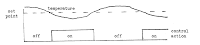
Temperature - On/off control
On/off control ( thermostat )
Occasionally known as two-step control, this is the
most basic control mode.
At point A (59°C, Figure ) the thermostat switches on, directing
the valve wide open. It takes time for the transfer of heat from the coil
to affect the water temperature, as shown by the graph of the water
temperature in Figure At point B (61°C) the thermostat switches
off and allows the valve to shut. However the coil is still full of steam,
which continues to condense and give up its heat. Hence the water
temperature continues to rise above the upper switching temperature,
and 'overshoots' at C, before eventually falling.
 From this point onwards, the water temperature in the tank continues
to fall until, at point D (59°C), the thermostat tells the valve to open.
Steam is admitted through the coil but again, it takes time to have an
effect and the water temperature continues to fall for a while, reaching
its trough of undershoot at point E.
The difference between the peak and the trough is known as the
operating differential. The switching differential of the thermostat
depends on the type of thermostat used. The operating differential
depends on the characteristics of the application such as the tank,
its contents, the heat transfer characteristics of the coil, the rate at
which heat is transferred to the thermostat, and so on.
Essentially, with on/off control, there are upper and lower switching
limits, and the valve is either fully open or fully closed - there is no

Occasionally known as two-step control, this is the
most basic control mode.
At point A (59°C, Figure ) the thermostat switches on, directing
the valve wide open. It takes time for the transfer of heat from the coil
to affect the water temperature, as shown by the graph of the water
temperature in Figure At point B (61°C) the thermostat switches
off and allows the valve to shut. However the coil is still full of steam,
which continues to condense and give up its heat. Hence the water
temperature continues to rise above the upper switching temperature,
and 'overshoots' at C, before eventually falling.
 From this point onwards, the water temperature in the tank continues
to fall until, at point D (59°C), the thermostat tells the valve to open.
Steam is admitted through the coil but again, it takes time to have an
effect and the water temperature continues to fall for a while, reaching
its trough of undershoot at point E.
The difference between the peak and the trough is known as the
operating differential. The switching differential of the thermostat
depends on the type of thermostat used. The operating differential
depends on the characteristics of the application such as the tank,
its contents, the heat transfer characteristics of the coil, the rate at
which heat is transferred to the thermostat, and so on.
Essentially, with on/off control, there are upper and lower switching
limits, and the valve is either fully open or fully closed - there is no
intermediate state.However, controllers are available that provide
a proportioning time
control, in which it is possible to alter the ratio of the 'on' time to the
'off' time to control the controlled condition. This proportioning action
occurs within a selected bandwidth around the set point; the set
point being the bandwidth mid point.
More
ON/OFF or two-position control
In many control applications it is satisfactory for the controller to
operate at either of two levels rather than over a continuous range.
In many applications the two levels are simple ON/OFF, e.g. valve
open or closed. However, the two levels may not be ON/OFF
control, in which it is possible to alter the ratio of the 'on' time to the
'off' time to control the controlled condition. This proportioning action
occurs within a selected bandwidth around the set point; the set
point being the bandwidth mid point.
More
ON/OFF or two-position control
In many control applications it is satisfactory for the controller to
operate at either of two levels rather than over a continuous range.
In many applications the two levels are simple ON/OFF, e.g. valve
open or closed. However, the two levels may not be ON/OFF

The major disadvantage with this type of control is that the controller
output bears no relationship to the error signal, i.e. the output is
ON/OFF or level 1 or level 2 no matter how high the error. The control
is either non or too much. In addition depending upon the sensitivity
of the system the controller may well cycle at high frequency, e.g. the
boiler being switched ON/OFF very rapidly as the temperature falls
and rises. To prevent this many controllers have ‘backlash’ built in or
have two limits provided. For example a room thermostat may be set
to 700F and due to backlash it will switch on a 680F and off at 720F.
This prevents the boiler being switched ON/OFF very rapidly if the
deviation around the set point was small. In addition theoretical analysis
of such a control system is difficult, i.e. the control action is
discontinuous, and is often treated as two linear problems (i) with the
system ON (ii) with the system OFF.
more
Bang bang control
How much should the software increase or decrease the drive signal?
One option is to just set the drive signal to its minimum value when you
want the plant to decrease its activity and to its maximum value when
you want the plant to increase its activity. This strategy is called on-off
control, and it is how many thermostats work.
more
Bang bang control
How much should the software increase or decrease the drive signal?
One option is to just set the drive signal to its minimum value when you
want the plant to decrease its activity and to its maximum value when
you want the plant to increase its activity. This strategy is called on-off
control, and it is how many thermostats work.

On-off control doesn't work well in all systems. If the thermostat waits
until the desired temperature is achieved to turn off the heater,
the temperature may overshoot. See Figure. The same amount of
overshoot and ripple probably isn't acceptable in an elevator.
more
until the desired temperature is achieved to turn off the heater,
the temperature may overshoot. See Figure. The same amount of
overshoot and ripple probably isn't acceptable in an elevator.
more
On-off Process control
On-off Process control


On-off control has two states: fully off and fully on. To prevent rapid
cycling, some hysteresis is added to the switching function. In operation,
the controller output is on from startup until temperature setpoint is
achieved. After overshoot, the temperature then falls to the hysteresis
limit, where power is reapplied On-off control can be used where:
- Where some temperature oscillation is permissible.
- The process is underpowered and the heater has little storage capacity.
- On electromechanical systems (compressors) where cycling must be
minimized
more
cycling, some hysteresis is added to the switching function. In operation,
the controller output is on from startup until temperature setpoint is
achieved. After overshoot, the temperature then falls to the hysteresis
limit, where power is reapplied On-off control can be used where:
- Where some temperature oscillation is permissible.
- The process is underpowered and the heater has little storage capacity.
- On electromechanical systems (compressors) where cycling must be
minimized
more

On-Off control has two states, fully off and fully on. To prevent rapid
cycling, some hysteresis is added to the switching function. In
operation, the controller output is on from start-up until temperature
set value is achieved. After overshoot, the temperature then falls to
the hysteresis limit and power is reapplied.
On-Off control can be used where:
- The process is underpowered and the heater has very little
storage capacity.
- Where some temperature oscillation is permissible.
- On electromechanical systems (compressors) where cycling
must be minimized
more
cycling, some hysteresis is added to the switching function. In
operation, the controller output is on from start-up until temperature
set value is achieved. After overshoot, the temperature then falls to
the hysteresis limit and power is reapplied.
On-Off control can be used where:
- The process is underpowered and the heater has very little
storage capacity.
- Where some temperature oscillation is permissible.
- On electromechanical systems (compressors) where cycling
must be minimized
more
ON-OFF Control Simulation
Temperature Controller Simulation
Instructions
The parameters are described elsewhere, with links to explanations
and definitions in the main document. Their values in the boxes can be
edited in the usual way. With the present values the set-point
temperature Ts will stay at 150 °C until 100 s into the simulation when
it will ramp linearly to 175 °C at 200 s. Either On-Off or PID controllers
can be selected with the first menu which also has an option
"PID Bode" to display the frequency-domain response of the PID
system. The second menu changes the temperature units.

more
on-off control elements
Universal Framework for Science and Engineering - Part 3:
Control systems. Processing of signals.
A lot of control systems use on-off control elements that have
the following in-out function
If we have several sets of photos of a 3D object, we can obtain
its 6D position. In this example, the problem is solved in the
following way. From the photos and virtual cameras, we obtain
the contours of the object as it is presented in the following
picture:
 more
more
Bang-Bang Control Using Temporal Logic
Simulation
This demonstration shows how to use Stateflow® to model
a bang-bang temperature control system for a boiler. The boiler
dynamics are modeled in Simulink® in a boiler plant model
Simulation Results
Looking at the Simulink scope, we can see that after
Instructions
The parameters are described elsewhere, with links to explanations
and definitions in the main document. Their values in the boxes can be
edited in the usual way. With the present values the set-point
temperature Ts will stay at 150 °C until 100 s into the simulation when
it will ramp linearly to 175 °C at 200 s. Either On-Off or PID controllers
can be selected with the first menu which also has an option
"PID Bode" to display the frequency-domain response of the PID
system. The second menu changes the temperature units.

more
on-off control elements
Universal Framework for Science and Engineering - Part 3:
Control systems. Processing of signals.
A lot of control systems use on-off control elements that have
the following in-out function
If we have several sets of photos of a 3D object, we can obtain
its 6D position. In this example, the problem is solved in the
following way. From the photos and virtual cameras, we obtain
the contours of the object as it is presented in the following
picture:
 more
moreBang-Bang Control Using Temporal Logic
Simulation
This demonstration shows how to use Stateflow® to model
a bang-bang temperature control system for a boiler. The boiler
dynamics are modeled in Simulink® in a boiler plant model
Simulation Results
Looking at the Simulink scope, we can see that after
approximately 450 seconds, the boiler temperature is effectively
maintained at the set temperature of 20 degrees Celsius.

Subscribe to:
Posts (Atom)


