Video Lecture Introduction To CNC Machines
Video Lecture Contour generation and Motion Control
Video Lecture Flow Control Valves
Showing posts with label Servo Motion Control. Show all posts
Showing posts with label Servo Motion Control. Show all posts
Tuesday, December 15, 2009
Tuesday, April 28, 2009
servo motor control-Velocity Profiling
A velocity profile is a graph of the velocity of a motor vs. time. The area inside the curve that the velocity profile creates is the distance traveled. Velocity profiling is useful for applications where specific velocities are necessary at specific times. Two typical velocity profiles are shown in the following figures.


These two figures are both examples of velocity profiles that can be implemented using the FlexMotion hardware and software. In the first example, the motor simply accelerates to a target velocity at a specified acceleration, runs at the target velocity, and then decelerates after a certain amount of time. In the second example, the motor accelerates to a certain velocity, runs at that target velocity for a period of time, accelerates to a higher velocity, then travels at that velocity for a period of time, and then decelerates to zero.
National Instruments - Fundamentals of Motion Control
http://zone.ni.com/devzone/cda/tut/p/id/3367
Creation of velocity profile using s-curves
In this paper an approach is proposed for velocity profile control of an AC motor. The dynamic control algorithms for calculation and estimation of the S-curve profile adapt in real time to variations in system behavior to improve their performance.
The S-curve velocity profile is similar to trapezoidal, and in this case, trapezium sides are replaced by S-curves, which enables smoother velocity transitions in acceleration and deceleration periods [1, 9].
The first order trapezoidal velocity profile is a typical point-to-point move. An
axis accelerates from rest to a given velocity at a constant rate. Then traverses, or slews, to a certain point where it decelerates at a constant rate until finally, the end position is reached and the axis will come to a rest. Sometimes the slew velocity and the end position can be changed on the fly. The S-curve velocity profile can be represented as a second-order polynomial in velocity. We have an extra term here – jerk (jerk is a derivative of acceleration and a measure of impact). The second order S-curve provides complete flexibility in the control of profiles for smoothing motion and eliminating jerk from mechanical systems. The degree of S-curve on a motion
profile is controlled by separate acceleration and deceleration smoothing (jerk-limit) factors.

Thursday, April 23, 2009
Servo Motor Motion Profiles - S-Curve
All servo systems consist of some kind of movement of a load. The method in which the load is moved is known as the motion profile. A motion profile can be as simple as a movement from point A to point B on a single axis
The S-curve motion profile allows for a gradual change in acceleration. This helps to reduce or eliminate the problems caused from overshoot, and the result is a great deal less mechanical vibration seen by the system. The minimum acceleration points occur at the beginning and end of the acceleration period, while the maximum acceleration occurs between these two points. This gives a motion profile that is fast and accurate.

The S-curve motion profile allows for a gradual change in acceleration. This helps to reduce or eliminate the problems caused from overshoot, and the result is a great deal less mechanical vibration seen by the system. The minimum acceleration points occur at the beginning and end of the acceleration period, while the maximum acceleration occurs between these two points. This gives a motion profile that is fast and accurate.

advancedmotioncontrols
http://www.advancedmotioncontrols.com
http://www.advancedmotioncontrols.com
Thursday, April 2, 2009
Servo motor control - Feedforward with PIV control
Fundamentals of servo motion control
Feedforward control
That missing ingredient provided we have access to both
Velocity and acceleration commands, synched up with
position commands is feedforward control.
An example of how feedforward control may be used in
parallel with disturbance rejection control is shown
in figure 8. The key is to accurately calculate the amount
of torque required to make each move a priori. To do so,
we take the basic equation of motion
 and approximate it (as follows) because the disturbance
torque Td is unknown.

more pdf
Fundamentals of Servo Motion Control
Feedforward Control
In order to achieve near zero following or tracking error,
feedforward control is often employed. A requirement for
feedforward control is the availability of both the velocity,
and acceleration, commands synchronized with the
position commands,. An example of how feedforward
control is used in addition to disturbance rejection control is
shown in Fig. 8.

Wednesday, April 1, 2009
AC Servo Motor Control Algorithm
A precise control of AC servo motor using neural
network PID controller
A new control technique based on a neural network, is proposed
here for control of AC servo motors. The PID control is widely
used in servo systems as it has simple structure, safety and
reliability. However, it has certain problems in a complex system,
resulting in imperfect action in the presence of uncertain
parameters. To solve these problems, a new hybrid control
algorithm of the PID controller is proposed, which could
prove the adequacy of the proposed control algorithm through
simulation and experiments after driving the AC
servo motor system using neural network PID controller.
Structure of PID controller using neural network control
 more pdf
Position Control of an AC Servo Motor Using
VHDL & FPGA
Abstract
In this paper, a new method of controlling position of
AC Servomotor using Field Programmable Gate Array (FPGA).
FPGA controller is used to generate direction and the number of
pulses required to rotate for a given angle. Pulses are sent as a square
wave, the number of pulses determines the angle of rotation and
frequency of square wave determines the speed of rotation. The
proposed control scheme has been realized using XILINX FPGA
SPARTAN XC3S400 and tested using MUMA012PIS model
Alternating Current (AC) servomotor. Experimental results show that
the position of the AC Servo motor can be controlled effectively.
INTRODUCTION
A servo motor is an Electro-mechanical device in which the
electrical input determines the position of the armature of
a motor. The shaft of the servo motor can be positioned to a
specific angle by sending the coded signal. The AC servo
motors have been widely used in the industrial fields and
various approaches have been made to realize high
performance motion control. These can be effectively utilized
in many position control systems subjected to external
disturbances such as friction.
With successively improving reliability and performance of
digital controllers, the digital control techniques have
predominated over other analog counter parts. The advantages
of digital controllers are:
• Reconfigurability
• Power saving options
• Less external passive components
• Less sensitive to temperature variation
• High efficiency


Abstract
This paper presents a Xilinx Field Programmable Gate Array
(FPGA) based speed control of AC Servomotor using sinusoidal
PWM technique. Xilinx FPGA is a programmable logic device
developed by Xilinx which is considered as an efficient hardware
for rapid prototyping. It is used to generate 50 Hz sine wave, the
triangular wave and the sinusoidal PWM signals. The sinusoidal
pulse width controls the speed of Motor. The proposed control
scheme has been realized using Xilinx FPGA SPARTAN
XC3S400 and tested using SM115 model Alternating Current
(AC) servomotor. The result provides a controllable speed with
satisfactory dynamic and static performances.
network PID controller
A new control technique based on a neural network, is proposed
here for control of AC servo motors. The PID control is widely
used in servo systems as it has simple structure, safety and
reliability. However, it has certain problems in a complex system,
resulting in imperfect action in the presence of uncertain
parameters. To solve these problems, a new hybrid control
algorithm of the PID controller is proposed, which could
prove the adequacy of the proposed control algorithm through
simulation and experiments after driving the AC
servo motor system using neural network PID controller.
Structure of PID controller using neural network control
more pdfPosition Control of an AC Servo Motor Using
VHDL & FPGA
Abstract
In this paper, a new method of controlling position of
AC Servomotor using Field Programmable Gate Array (FPGA).
FPGA controller is used to generate direction and the number of
pulses required to rotate for a given angle. Pulses are sent as a square
wave, the number of pulses determines the angle of rotation and
frequency of square wave determines the speed of rotation. The
proposed control scheme has been realized using XILINX FPGA
SPARTAN XC3S400 and tested using MUMA012PIS model
Alternating Current (AC) servomotor. Experimental results show that
the position of the AC Servo motor can be controlled effectively.
INTRODUCTION
A servo motor is an Electro-mechanical device in which the
electrical input determines the position of the armature of
a motor. The shaft of the servo motor can be positioned to a
specific angle by sending the coded signal. The AC servo
motors have been widely used in the industrial fields and
various approaches have been made to realize high
performance motion control. These can be effectively utilized
in many position control systems subjected to external
disturbances such as friction.
With successively improving reliability and performance of
digital controllers, the digital control techniques have
predominated over other analog counter parts. The advantages
of digital controllers are:
• Reconfigurability
• Power saving options
• Less external passive components
• Less sensitive to temperature variation
• High efficiency

more ( pdf )
New Digital Hardware Control Method for High
Performance AC Servo Motor
Abstract:
Today’s motor drives widely use Digital Signal
Processor (DSP) or Microcontroller to
implement the digital control algorithm. Most
recently new requirements have arisen. These
include faster torque control update with flexible
design capability of motion peripherals for high
performance military servo drive applications.
A Complete digital hardware based AC servo
drive development system has been developed to
satisfy increasing demand for performance
enhancement. Based on the FPGA, the system is
configurable for either induction or permanent
magnet machine servo control. The detail design
of complete hardware based high performance
AC servo drive system is discussed.

Control Block Diagram
more pdf
FPGA Based Speed Control of AC Servomotor
Using Sinusoidal PWM
more pdf
FPGA Based Speed Control of AC Servomotor
Using Sinusoidal PWM
Abstract
This paper presents a Xilinx Field Programmable Gate Array
(FPGA) based speed control of AC Servomotor using sinusoidal
PWM technique. Xilinx FPGA is a programmable logic device
developed by Xilinx which is considered as an efficient hardware
for rapid prototyping. It is used to generate 50 Hz sine wave, the
triangular wave and the sinusoidal PWM signals. The sinusoidal
pulse width controls the speed of Motor. The proposed control
scheme has been realized using Xilinx FPGA SPARTAN
XC3S400 and tested using SM115 model Alternating Current
(AC) servomotor. The result provides a controllable speed with
satisfactory dynamic and static performances.

Saturday, March 28, 2009
Servo Motion Control
Control
Servo Motion Control - PID Control
Servo Motion Control - PIV Control
DC Servo motor control
AC Servo Motor Control Algorithm
Servo motor control - Feedforward with PIV control
Tuning
Servo Motion Control Tuning the PID Loop
Modeling
MODELING OF A DC SERVOMOTOR
System Modeling - Linear Permanent Magnet Motors
Servo Motion Control Tuning the PID Loop
There are two primary ways to go about selecting the PID gains.
Either the operator uses a trial and error or an analytical approach.
Using a trial and error approach relies significantly on the
operator’s own prior experience with other servo systems. The one
significant downside to this is that there is no physical insight into
what the gains mean and there is no way to know if the gains are
optimum by any definition. However, for decades this was the
approach most commonly used. In fact, it is still used
today for low performance systems usually found in process control.
To address the need for an analytical approach, Ziegler and Nichols
[1] proposed a method based on their many years of industrial
control experience. Although they originally intended their tuning
method for use in process control, their technique can be applied to
servo control. Their procedure basically boils down to these two steps.
Step 1:
Set Ki and Kd to zero. Excite the system with a step command.
Slowly increase Kp until the shaft position begins to oscillate.
At this point, record the value of Kp and set Ko equal to this value.
Record the oscillation frequency, fo.
Step 2:
Set the final PID gains using equation (6).
 Loosely speaking, the proportional term affects the overall response
of the system to a position error. The integral term is needed to force
the steady state position error to zero for a constant position
command and the derivative term is needed to provide a damping
action, as the response becomes oscillatory. Unfortunately all three
parameters are inter-related so that by adjusting one parameter will
effect any of a previous parameter adjustments. As an example of
this tuning approach, we investigate the response of a Compumotor
BE342A motor with a generic servo drive and controller.
This servomotor has the following parameters:
Motor Total Inertia J = 50E-6 kgm^2
Motor Damping b = .1E-3 Nm/ (rad/sec)
Torque Constant Kt = .6 Nm/A
We begin with observing the response to a step input command with
no disturbance torque (Td = 0).
Step 1:
Fig. 2a shows the result of slowly increasing only the proportional term.
The system begins to oscillate at approximately .5 Hz (fo = .5Hz) with
Ko of approximately 5E-5 Nm/ rad.
Step 2:
Using these values, the optimum P.I .D. gains according to
Ziegler-Nichols (Z-N) are then (using equation (6)):
Kp = 3.0E-4 Nm/ rad
Ki = 3.0E-4 Nm/ (rad/sec)
Kd = 7.4E-5 Nm/ (rad/sec)
Fig. 2b shows the result of using the Ziegler Nichols gains.
The response is somewhat better than just a straight proportional gain.
As a comparison, other gains were obtained by trial and error. One set
Of additional gains is listed in Fig. 2b. Although the trial and error gains
gave a faster, less oscillatory response, there is no way of telling if a
better solution exits without further exhaustive testing.

One characteristic that is very apparent in Fig.2 is the length of
the settling time. The system using Ziegler Nichols takes about
6 seconds to finally settle making it very difficult to incorporate
into any highperformance motion control application. In contrast,
the trial and error settings gives a quicker settling time, however
no solution was found to completely remove the overshoot.
Source ( pdf )
http://www.compumotor.com/whitepages/ServoFundamentals.pdf
Friday, March 27, 2009
DC Servo motor control
NEURAL ADAPTIVE TACKING CONTROL OF A
LOW SPEED DC SERVO SYSTEM
Hu Hongjie Chen Jingquan Er Lianjie
DC SERVO SYSTEM
The low speed system’s hardware setup is composed of a
permanent dc motor, driving circuit, servo amplifier
(PWM), a mechanical frame as an inertial load, interface
circuit (A/D and D/A), an encoder for position sensing,
and a personal computer (PETIUM I 133) is used as the
programming environment, using Borlandc31 as
programming language for the real-time control
application. Sampling time is defined as 5ms. The block
diagram of the hardware setup is shown in figure

more ( pdf )
Two Adaptive Friction Compensation for DC Servomotors
Abstract
Two advanced control strategies of adaptive friction
Compensation For DC servomotor are presented in this paper,
the first is used for The direct on-line friction compensation in
the velocity control system, The second is making use of an
adaptive inverse neural network controller In the position control
system. Both are composed of an adaptive Compensator for
the nonlinear stiction and Coulomp friction in Parallel with a
PID regulator. Experiments show that much improvement
Of performance has attained respect to conventional controller

more ( pdf )
Feedforward and IMP Control Applied to a DC Servo Motor
Feedforward and IMP Control Applied to a DC Servo Motor
1.0 Introduction
The purpose of this report is to compare feedforward and internal
model principle (IMP) control applied to a DC servo motor.
These control schemes will be tested with known sinusoidal inputs.
The performance of the control schemes will be compared to the
Open loop performance of the system. System identification of
the motor is another task that will be performed.
Feedforward Control
Feedforward control was implemented by inverting (2) to yield:

this gives an overall transfer function of one for the system as
can be seen from figure 3. Even though H(s) is not a proper
transfer function, the control system could be implemented
because the input signal is a known sine wave so the first and
second derivatives can be readily calculated.
can be seen from figure 3. Even though H(s) is not a proper
transfer function, the control system could be implemented
because the input signal is a known sine wave so the first and
second derivatives can be readily calculated.

Internal Model Principle Control (IMP)
The internal model principle [Control System Design, Goodwin
et. al.] can be used to design a controller when the input to the
system is know and can be modeled in the Laplace domain.
The internal model principle [Control System Design, Goodwin
et. al.] can be used to design a controller when the input to the
system is know and can be modeled in the Laplace domain.

more ( pdf )
MODELLING AND CONTROL OF A DC SERVO MOTOR
WITH LABVIEW
MODELLING AND CONTROL OF A DC SERVO MOTOR
WITH LABVIEW
OBJECTIVES
This is a hands-on session on the application of computer-based
control to a voltage-controllable electro-mechanical system – the
DC motor. The session is mainly concerned with the modelling
and control of a DC servo motor system, fully instrumented with
position and velocity measurements. National Instrument’s
LabVIEW will be the control software for the experiment. At the
end of the experiment, you should have some experience in
• Simple static and dynamic modelling of the DC motor system,
• Manual and feedback control of the system for velocity tracking
To benefit more fully from this session, students should read the
manual and answer the pre-laboratory questions (Q1-Q3) before
going to the laboratory.

Fig1. DC Servomotor
More pdf
Real –Time DC Motor Position Control by Fuzzy Logic
and PID Controllers Using Labview
Abstract
This paper presents the position control of a DC
motor using Fuzzy Logic and PID Control algorithms. Fuzzy
Logic and PID controllers are designed based on labview
program, and the real - time position control of the DC motor
was realized by using DAQ device. The experimental results
demonstrate that the responses of DC motor with FLC show a
satisfactory, well damped control performance.

Fig .3. The block diagram of proposed PID Controller structure
More pdf
DC Servomotor Controller
This is an experiment on the closed loop DC servomotor control
system (SMC). It will able to be used for practical use with/without
some modifications. The closed loop servo mechanism requires
real-time servo operations, such as position control, velocity
control and torque control. It will be suitable for implementation
to any embedded 32 bit RISC processors as a middleware. In this
project, these operations are processed with only a cheap 8 bit
microcontroller.

Friday, March 20, 2009
Servo Motion - Control PIV Control
In order to be able to better predict the system response, an
alternative topology is needed. One example of an easier to
tune topology is the PIV controller shown in Fig.3. This
controller basically combines a position loop with a velocity loop.
More specifically, the result of the position error multiplied
by Kp becomes a velocity correction command. The integral
term, Ki now operates directly on the velocity error instead of
the position error as in the PID case and finally, the Kd term
in the PID position loop is replaced by a Kv term in the PIV
velocity loop. Note however, they have the same units,
Nm/ (rad/sec).

PIV control requires the knowledge of the motor velocity,
labeled velocity estimator in Fig.3. This is usually formed by
a simple filter, however significant delays can result and must
be accounted for if truly accurate responses are needed.
Alternatively, the velocity can be obtained by use of a velocity
observer. This observer requires the use of other state variables
in exchange for providing zero lag filtering properties. In either
case, a clean velocity signal must be provided for PIV control.
As an example of this tuning approach, we investigate the
response of a Compumotor Gemini series servo drive and built in
controller using the same motor from the previous example.
Again, we begin with observing the response to a step input
command with no external disturbance torque (Td = 0).
Tuning the PIV Loop
To tune this system, only two control parameters are needed,
the bandwidth (BW) and the damping ratio (z). An estimate
of the motor’s total inertia, ˆ J and damping, ˆ b are also required
at set-up and are obtained using the motor/drive set up utilities.
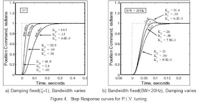
Figure 4 illustrates typical response plots for various bandwidths
and damping ratios.
labeled velocity estimator in Fig.3. This is usually formed by
a simple filter, however significant delays can result and must
be accounted for if truly accurate responses are needed.
Alternatively, the velocity can be obtained by use of a velocity
observer. This observer requires the use of other state variables
in exchange for providing zero lag filtering properties. In either
case, a clean velocity signal must be provided for PIV control.
As an example of this tuning approach, we investigate the
response of a Compumotor Gemini series servo drive and built in
controller using the same motor from the previous example.
Again, we begin with observing the response to a step input
command with no external disturbance torque (Td = 0).
Tuning the PIV Loop
To tune this system, only two control parameters are needed,
the bandwidth (BW) and the damping ratio (z). An estimate
of the motor’s total inertia, ˆ J and damping, ˆ b are also required
at set-up and are obtained using the motor/drive set up utilities.
Figure 4 illustrates typical response plots for various bandwidths
and damping ratios.

With the damping ratio fixed, the bandwidth directly relates to
the system rise time as shown in Fig.4 a). The higher the bandwidth,
the quicker the rise and settling times. Damping, on the other hand,
relates primary to overshoot and secondarily to rise time. The less
damping, the higher the overshoot and the slightly quicker the rise
time for a fixed bandwidth. This scenario is shown in Fig. 4 b).
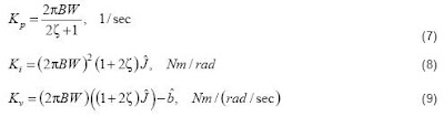
The actual internal PIV gains can be calculated directly from
the bandwidth and damping values along with the estimates of
the inertia, ˆ J and motor viscous damping, ˆ b , making their use
straightforward and easy to implement. The actual analytical
expressions are described in equations (7) - (9).
the system rise time as shown in Fig.4 a). The higher the bandwidth,
the quicker the rise and settling times. Damping, on the other hand,
relates primary to overshoot and secondarily to rise time. The less
damping, the higher the overshoot and the slightly quicker the rise
time for a fixed bandwidth. This scenario is shown in Fig. 4 b).
The actual internal PIV gains can be calculated directly from
the bandwidth and damping values along with the estimates of
the inertia, ˆ J and motor viscous damping, ˆ b , making their use
straightforward and easy to implement. The actual analytical
expressions are described in equations (7) - (9).

In reality, the user never wants to put a step command into their
mechanics, unless of course the step is so small that no damage
will result. The use of a step response in determining a system’s
performance is mostly traditional. The structure of the PIV
control and for that matter, the PID control is designed to reject
unknown disturbances to the system. Fig.1 shows this unknown
torque disturbance, Td as part of the servo motor model.
Source ( pdf )
http://www.compumotor.com/whitepages/ServoFundamentals.pdf
Thursday, March 19, 2009
Servo Motion Control - PID Control
PID position loops
Theory
The velocity loop is the most basic servo control loop. However,
since a velocity loop cannot ensure that the machine stays in
position over long periods of time, most applications require
position control. There are two common configurations used for
position control: the cascaded position-velocity loop, as discussed
last month, and the PID position controller, as shown below.

Block diagram of PID position loop
The position loop compares a position command to a position
feedback signal, and calculates the position error, PE. In a PID
controller, current command is generated with three gains: PE is
scaled by the proportional gain (KPP), the integral of PE is scaled by
the integral gain (KPI), and the derivative of PE is scaled by the
derivative gain (KPD).
More ( pdf )
http://apps.danahermotion.com/support/troubleshooting/
PDF_Resources/2000-08%20PID%20pos%20loops.pdf
Servo Motion Control - PID Control
Theory
The velocity loop is the most basic servo control loop. However,
since a velocity loop cannot ensure that the machine stays in
position over long periods of time, most applications require
position control. There are two common configurations used for
position control: the cascaded position-velocity loop, as discussed
last month, and the PID position controller, as shown below.
Block diagram of PID position loop
The position loop compares a position command to a position
feedback signal, and calculates the position error, PE. In a PID
controller, current command is generated with three gains: PE is
scaled by the proportional gain (KPP), the integral of PE is scaled by
the integral gain (KPI), and the derivative of PE is scaled by the
derivative gain (KPD).
More ( pdf )
http://apps.danahermotion.com/support/troubleshooting/
PDF_Resources/2000-08%20PID%20pos%20loops.pdf
Servo Motion Control - PID Control
The basic components of a typical servo motion system are
depicted in Fig.1 using standard LaPlace notation. In this figure,
the servo drive closes a current loop and is modeled simply as
a linear transfer function G(s). Of course the servo drive will
have peak current limits, so this linear model is not entirely
accurate, however it does provide a reasonable representation
for our analysis. In their most basic form, servo drives receive
a voltage command that represents a desired motor current.
Motor shaft torque, T is related to motor current, I by the torque
constant, Kt. Equation (1) shows this relationship.
 For the purposes of this discussion the transfer function of
the current regulator or really the torque regulator can be
approximated as unity for the relatively lower motion frequencies
we are interested in and therefore we make the following
approximation shown in (2).
 The servomotor is modeled as a lump inertia, J, a viscous damping
term, b, and a torque constant, Kt. The lump inertia term is
comprised of both the servomotor and load inertia. I t is also
assumed that the load is rigidly coupled such that the torsional
rigidity moves the natural mechanical resonance point well
out beyond the servo controller’s bandwidth. This assumption
allows us to model the total system inertia as the sum of the
motor and load inertia for the frequencies we can control.
Somewhat more complicated models are needed if coupler
dynamics are incorporated.
The actual motor position, q(s) is usually measured by either an
encoder or resolver coupled directly to the motor shaft. Again the
underlying assumption is that the feedback device is rigidly
mounted such that its mechanical resonant frequencies can be
safely ignored. External shaft torque disturbances, Td are added
to the torque generated by the motor's current to give the torque
available to accelerate the total inertia, J.

 There are three gains to adjust in the PID controller, Kp, Ki and Kd.
These gains all act on the position error defined in (4). Note the
superscript "* " refers to a commanded value.
 The output of the PID controller is a torque signal. I ts mathematical
expression in the time domain is given in (5).

depicted in Fig.1 using standard LaPlace notation. In this figure,
the servo drive closes a current loop and is modeled simply as
a linear transfer function G(s). Of course the servo drive will
have peak current limits, so this linear model is not entirely
accurate, however it does provide a reasonable representation
for our analysis. In their most basic form, servo drives receive
a voltage command that represents a desired motor current.
Motor shaft torque, T is related to motor current, I by the torque
constant, Kt. Equation (1) shows this relationship.
 For the purposes of this discussion the transfer function of
the current regulator or really the torque regulator can be
approximated as unity for the relatively lower motion frequencies
we are interested in and therefore we make the following
approximation shown in (2).
 The servomotor is modeled as a lump inertia, J, a viscous damping
term, b, and a torque constant, Kt. The lump inertia term is
comprised of both the servomotor and load inertia. I t is also
assumed that the load is rigidly coupled such that the torsional
rigidity moves the natural mechanical resonance point well
out beyond the servo controller’s bandwidth. This assumption
allows us to model the total system inertia as the sum of the
motor and load inertia for the frequencies we can control.
Somewhat more complicated models are needed if coupler
dynamics are incorporated.
The actual motor position, q(s) is usually measured by either an
encoder or resolver coupled directly to the motor shaft. Again the
underlying assumption is that the feedback device is rigidly
mounted such that its mechanical resonant frequencies can be
safely ignored. External shaft torque disturbances, Td are added
to the torque generated by the motor's current to give the torque
available to accelerate the total inertia, J.

Around the servo drive and motor block is the servo controller that
closes the position loop. A basic servo controller generally contains
both a trajectory generator and a PID controller. The trajectory
generator typically provides only position setpoint commands labeled
in Fig.1 as q* (s). The PID controller operates on the position error
and outputs a torque command that is sometimes scaled by an
estimate of the motor's torque constant, ˆt K . I f the motor's torque
constant is not known, the PID gains are simply re-scaled accordingly.
Because the exact value of the motor's torque constant is generally
not known, the symbol "^ " is used to indicate it is an estimated value
in the controller. In general, equation (3) holds with sufficient accuracy
so that the output of the servo controller (usually + / - 10 volts) will
command the correct amount of current for a desired torque.
 There are three gains to adjust in the PID controller, Kp, Ki and Kd.
These gains all act on the position error defined in (4). Note the
superscript "* " refers to a commanded value.
 The output of the PID controller is a torque signal. I ts mathematical
expression in the time domain is given in (5).

Source (pdf )
http://www.compumotor.com/whitepages/ServoFundamentals.pdf
Subscribe to:
Posts (Atom)

