Servo Motion Control

Control

Servo Motion Control - PID Control

Servo Motion Control - PIV Control

DC Servo motor control

AC Servo Motor Control Algorithm

Servo motor control - Feedforward with PIV control

Tuning

Servo Motion Control Tuning the PID Loop

Modeling

MODELING OF A DC SERVOMOTOR

System Modeling - Linear Permanent Magnet Motors

Servo Motion Control Tuning the PID Loop

There are two primary ways to go about selecting the PID gains.
Either the operator uses a trial and error or an analytical approach.
Using a trial and error approach relies significantly on the
operator’s own prior experience with other servo systems. The one
significant downside to this is that there is no physical insight into
what the gains mean and there is no way to know if the gains are
optimum by any definition. However, for decades this was the
approach most commonly used. In fact, it is still used
today for low performance systems usually found in process control.
To address the need for an analytical approach, Ziegler and Nichols
[1] proposed a method based on their many years of industrial
control experience. Although they originally intended their tuning
method for use in process control, their technique can be applied to
servo control. Their procedure basically boils down to these two steps.

Step 1:
Set Ki and Kd to zero. Excite the system with a step command.
Slowly increase Kp until the shaft position begins to oscillate.
At this point, record the value of Kp and set Ko equal to this value.
Record the oscillation frequency, fo.

Step 2:

Set the final PID gains using equation (6).



Loosely speaking, the proportional term affects the overall response

of the system to a position error. The integral term is needed to force
the steady state position error to zero for a constant position
command and the derivative term is needed to provide a damping
action, as the response becomes oscillatory. Unfortunately all three
parameters are inter-related so that by adjusting one parameter will
effect any of a previous parameter adjustments. As an example of
this tuning approach, we investigate the response of a Compumotor
BE342A motor with a generic servo drive and controller.

This servomotor has the following parameters:

Motor Total Inertia J = 50E-6 kgm^2
Motor Damping b = .1E-3 Nm/ (rad/sec)
Torque Constant Kt = .6 Nm/A

We begin with observing the response to a step input command with
no disturbance torque (Td = 0).

Step 1:
Fig. 2a shows the result of slowly increasing only the proportional term.
The system begins to oscillate at approximately .5 Hz (fo = .5Hz) with
Ko of approximately 5E-5 Nm/ rad.

Step 2:

Using these values, the optimum P.I .D. gains according to
Ziegler-Nichols (Z-N) are then (using equation (6)):

Kp = 3.0E-4 Nm/ rad
Ki = 3.0E-4 Nm/ (rad/sec)
Kd = 7.4E-5 Nm/ (rad/sec)

Fig. 2b shows the result of using the Ziegler Nichols gains.
The response is somewhat better than just a straight proportional gain.
As a comparison, other gains were obtained by trial and error. One set
Of additional gains is listed in Fig. 2b. Although the trial and error gains
gave a faster, less oscillatory response, there is no way of telling if a
better solution exits without further exhaustive testing.

One characteristic that is very apparent in Fig.2 is the length of
the settling time. The system using Ziegler Nichols takes about
6 seconds to finally settle making it very difficult to incorporate
into any highperformance motion control application. In contrast,
the trial and error settings gives a quicker settling time, however
no solution was found to completely remove the overshoot.

Source ( pdf )
http://www.compumotor.com/whitepages/ServoFundamentals.pdf

Control and Automation Home

DC Servo motor control

NEURAL ADAPTIVE TACKING CONTROL OF A
LOW SPEED DC SERVO SYSTEM

Hu Hongjie Chen Jingquan Er Lianjie

DC SERVO SYSTEM
The low speed system’s hardware setup is composed of a
permanent dc motor, driving circuit, servo amplifier
(PWM), a mechanical frame as an inertial load, interface
circuit (A/D and D/A), an encoder for position sensing,
and a personal computer (PETIUM I 133) is used as the
programming environment, using Borlandc31 as
programming language for the real-time control
application. Sampling time is defined as 5ms. The block
diagram of the hardware setup is shown in figure

more ( pdf )

Two Adaptive Friction Compensation for DC Servomotors

Abstract
Two advanced control strategies of adaptive friction
Compensation For DC servomotor are presented in this paper,
the first is used for The direct on-line friction compensation in
the velocity control system, The second is making use of an
adaptive inverse neural network controller In the position control
system. Both are composed of an adaptive Compensator for
the nonlinear stiction and Coulomp friction in Parallel with a
PID regulator. Experiments show that much improvement
Of performance has attained respect to conventional controller

more ( pdf )


Feedforward and IMP Control Applied to a DC Servo Motor

1.0 Introduction
The purpose of this report is to compare feedforward and internal
model principle (IMP) control applied to a DC servo motor.
These control schemes will be tested with known sinusoidal inputs.
The performance of the control schemes will be compared to the
Open loop performance of the system. System identification of
the motor is another task that will be performed.

Feedforward Control
Feedforward control was implemented by inverting (2) to yield:

this gives an overall transfer function of one for the system as
can be seen from figure 3. Even though H(s) is not a proper
transfer function, the control system could be implemented
because the input signal is a known sine wave so the first and
second derivatives can be readily calculated.

Internal Model Principle Control (IMP)
The internal model principle [Control System Design, Goodwin
et. al.] can be used to design a controller when the input to the
system is know and can be modeled in the Laplace domain.

more ( pdf )

MODELLING AND CONTROL OF A DC SERVO MOTOR
WITH LABVIEW

OBJECTIVES
This is a hands-on session on the application of computer-based
control to a voltage-controllable electro-mechanical system – the
DC motor. The session is mainly concerned with the modelling
and control of a DC servo motor system, fully instrumented with
position and velocity measurements. National Instrument’s
LabVIEW will be the control software for the experiment. At the
end of the experiment, you should have some experience in

• Simple static and dynamic modelling of the DC motor system,

• Manual and feedback control of the system for velocity tracking

To benefit more fully from this session, students should read the
manual and answer the pre-laboratory questions (Q1-Q3) before
going to the laboratory.

Fig1. DC Servomotor

More pdf



Real –Time DC Motor Position Control by Fuzzy Logic
and PID Controllers Using Labview

Abstract
This paper presents the position control of a DC
motor using Fuzzy Logic and PID Control algorithms. Fuzzy
Logic and PID controllers are designed based on labview
program, and the real - time position control of the DC motor
was realized by using DAQ device. The experimental results
demonstrate that the responses of DC motor with FLC show a
satisfactory, well damped control performance.

Fig .3. The block diagram of proposed PID Controller structure

More pdf

DC Servomotor Controller
This is an experiment on the closed loop DC servomotor control
system (SMC). It will able to be used for practical use with/without
some modifications. The closed loop servo mechanism requires
real-time servo operations, such as position control, velocity
control and torque control. It will be suitable for implementation
to any embedded 32 bit RISC processors as a middleware. In this
project, these operations are processed with only a cheap 8 bit
microcontroller.

Figure 5. Operation diagram for the SMC (Cascaded control)

more

Control and Automation Home

System Modeling - Linear Permanent Magnet Motors

Two types of position dependent disturbances are
considered: cogging force and force ripple. Cogging is
a magnetic disturbance force that is caused by attraction
between permanent magnets and translator. The force
depends on the relative position of the translator with
respect to the magnets, and it is independent of the motor
current. Force ripple is an electro-magnetic effect and
causes a periodic variation of the force constant c. Force
ripple occurs only if the motor current is different from
zero, and its absolute value depends on the required thrust
force and the relative position of the translator to the
stator. Both disturbances are periodic functions of the
position. [9]

Cogging is negligible in motors with iron-less translators
[14]. Figure 3 shows the nonlinear block diagram of a
servo system with brushless linear motor. The nonlinear
disturbances are the velocity depended friction force
Ffriction, and the position dependent cogging force
Fcogging and force ripple



The friction force is modeled with a kinetic friction
model. In the kinetic friction model the friction force is a
function of velocity only. The friction curve is identified
with experiments at different velocities. The friction has
a discontinuity at

because of stiction. Stiction
avoid accurate measurement of the thrust force without
motion of the carriage. A survey of friction models and
compensation methods is given in [17].
Aim of the force ripple identification is to obtain a
function of the thrust force Fthrust versus the control
signal u and the position x. A possible solution to identify
this function is to measure the thrust force Fthrust at
different positions x and control signals u. In this case an
additional force sensor and a screw cylinder for manual
position adjustment is necessary. In order to measure the
force ripple accurately, without motion of the carriage, a
frictionless air bearing support is necessary [7]. A solution
to avoid frictionless air bearings is the measurement of the
thrust force with moving carriage. At constant velocities
the friction force is also constant and can be treated as
additional load force. In this case an additional servo
system is needed to achieve the movement [18].

The main idea of the proposed identification method is
to identify the force ripple in a closed position control loop
by measuring the control signal u at different load forces
Fload and positions x. Neither additional force sensor nor
device for position adjustment are necessary. In order to
avoid inaccuracy by stiction the measurement is achieved
with moving carriage. The position of the carriage is
obtained from an incremental linear optical encoder with
a measurement resolution of 0:2m. The experiment
consists of several movements at constant low velocity
(1mm=s) and different load forces (0 : : : 70N). The
output of the position controller is stored at equidistant
positions. A controller with an integral component is used
to eliminate steady position error. During motion with
constant low velocity the dynamics of the motor have no
significant effect on the control signal u.

Figure 4 shows the controller output u versus the
translator position x. In this first experiment there is no
additional load force attached to the carriage. The period
spectrum of the controller signal ui is carried out via FFT.

Source ( pdf )

http://www.inf.fh-dortmund.de/personen/professoren/

roehrig/papers/ldia01.pdf

MODELING OF A DC SERVO MOTOR

MODELING OF A DC SERVO MOTOR
Electric motors are the most common actuator used in
electromagnetic systems of all types. They are made in a
variety of configurations and sizes for applications ranging
from activating precision movements to powering diesel-electric
locomotives. The laboratory motors are small servomotors,
which might be used for positioning control applications in a
variety of automated machines. They are DC (direct current)
motors. The armature is driven by an external DC voltage that
produces the motor torque and results in the motor speed. The
armature current produced by the applied voltage interacts with
the permanent magnet field to produce current and motion.
A simplified schematic of the motor is shown in Figure 1 below.

more

DC Servo Motor Parameter Estimation
This example demonstrates the process of estimating the
parameters of a multi-domain DC servo motor model constructed
using various physical modeling products.
Contents
1.Description of the DC Servo Motor System
2.Estimating Parameters of the DC Motor Model
3.Importing Experimental Data
4.Selecting Parameters for Estimation
5.Defining an Estimation
6.Running the Estimation
7.Validation
8.Summary

more


DC Motor System Identification
Objective The purpose of this lab is to experimentally determine
the frequency response of a DC servomotor system, which
includes the DC motor and amplifier. Experimental results will be
obtained to create a Bode plot for the servomotor system.
A transfer function can also be derived by fitting the Bode plot.
These results then can be used to design a suitable controller.

More pdf

On/off control

1. On/off control Simulator

2. On-off Process control

3. Temperature - On/off control

4. ON-OFF Control - refrigeration system




Control and Automation Home

Model and Friction Compensation

1. Model and Friction Compensation

2. Actuators Friction Compensation

3 Friction Compensation algorithms 1

4. Friction Compensation in position and speed control

5. Friction Modelling near Striebeck Velocities

Servo Motion - Control PIV Control

In order to be able to better predict the system response, an
alternative topology is needed. One example of an easier to
tune topology is the PIV controller shown in Fig.3. This
controller basically combines a position loop with a velocity loop.
More specifically, the result of the position error multiplied
by Kp becomes a velocity correction command. The integral
term, Ki now operates directly on the velocity error instead of
the position error as in the PID case and finally, the Kd term
in the PID position loop is replaced by a Kv term in the PIV
velocity loop. Note however, they have the same units,
Nm/ (rad/sec).

PIV control requires the knowledge of the motor velocity,
labeled velocity estimator in Fig.3. This is usually formed by
a simple filter, however significant delays can result and must
be accounted for if truly accurate responses are needed.
Alternatively, the velocity can be obtained by use of a velocity
observer. This observer requires the use of other state variables
in exchange for providing zero lag filtering properties. In either
case, a clean velocity signal must be provided for PIV control.
As an example of this tuning approach, we investigate the
response of a Compumotor Gemini series servo drive and built in
controller using the same motor from the previous example.
Again, we begin with observing the response to a step input
command with no external disturbance torque (Td = 0).

Tuning the PIV Loop
To tune this system, only two control parameters are needed,
the bandwidth (BW) and the damping ratio (z). An estimate
of the motor’s total inertia, ˆ J and damping, ˆ b are also required
at set-up and are obtained using the motor/drive set up utilities.
Figure 4 illustrates typical response plots for various bandwidths
and damping ratios.

With the damping ratio fixed, the bandwidth directly relates to
the system rise time as shown in Fig.4 a). The higher the bandwidth,
the quicker the rise and settling times. Damping, on the other hand,
relates primary to overshoot and secondarily to rise time. The less
damping, the higher the overshoot and the slightly quicker the rise
time for a fixed bandwidth. This scenario is shown in Fig. 4 b).
The actual internal PIV gains can be calculated directly from
the bandwidth and damping values along with the estimates of
the inertia, ˆ J and motor viscous damping, ˆ b , making their use
straightforward and easy to implement. The actual analytical
expressions are described in equations (7) - (9).

In reality, the user never wants to put a step command into their
mechanics, unless of course the step is so small that no damage
will result. The use of a step response in determining a system’s
performance is mostly traditional. The structure of the PIV
control and for that matter, the PID control is designed to reject
unknown disturbances to the system. Fig.1 shows this unknown
torque disturbance, Td as part of the servo motor model.

Source ( pdf )
http://www.compumotor.com/whitepages/ServoFundamentals.pdf

Control and Automation Home

Servo Motion Control - PID Control

PID position loops

Theory
The velocity loop is the most basic servo control loop. However,
since a velocity loop cannot ensure that the machine stays in
position over long periods of time, most applications require
position control. There are two common configurations used for
position control: the cascaded position-velocity loop, as discussed
last month, and the PID position controller, as shown below.


Block diagram of PID position loop
The position loop compares a position command to a position
feedback signal, and calculates the position error, PE. In a PID
controller, current command is generated with three gains: PE is
scaled by the proportional gain (KPP), the integral of PE is scaled by
the integral gain (KPI), and the derivative of PE is scaled by the
derivative gain (KPD).

More ( pdf )
http://apps.danahermotion.com/support/troubleshooting/
PDF_Resources/2000-08%20PID%20pos%20loops.pdf

Servo Motion Control - PID Control

The basic components of a typical servo motion system are
depicted in Fig.1 using standard LaPlace notation. In this figure,
the servo drive closes a current loop and is modeled simply as
a linear transfer function G(s). Of course the servo drive will
have peak current limits, so this linear model is not entirely
accurate, however it does provide a reasonable representation
for our analysis. In their most basic form, servo drives receive
a voltage command that represents a desired motor current.
Motor shaft torque, T is related to motor current, I by the torque
constant, Kt. Equation (1) shows this relationship.

For the purposes of this discussion the transfer function of
the current regulator or really the torque regulator can be
approximated as unity for the relatively lower motion frequencies
we are interested in and therefore we make the following
approximation shown in (2).

The servomotor is modeled as a lump inertia, J, a viscous damping
term, b, and a torque constant, Kt. The lump inertia term is
comprised of both the servomotor and load inertia. I t is also
assumed that the load is rigidly coupled such that the torsional
rigidity moves the natural mechanical resonance point well
out beyond the servo controller’s bandwidth. This assumption
allows us to model the total system inertia as the sum of the
motor and load inertia for the frequencies we can control.
Somewhat more complicated models are needed if coupler
dynamics are incorporated.

The actual motor position, q(s) is usually measured by either an
encoder or resolver coupled directly to the motor shaft. Again the
underlying assumption is that the feedback device is rigidly
mounted such that its mechanical resonant frequencies can be
safely ignored. External shaft torque disturbances, Td are added
to the torque generated by the motor's current to give the torque
available to accelerate the total inertia, J.

Around the servo drive and motor block is the servo controller that
closes the position loop. A basic servo controller generally contains
both a trajectory generator and a PID controller. The trajectory
generator typically provides only position setpoint commands labeled
in Fig.1 as q* (s). The PID controller operates on the position error
and outputs a torque command that is sometimes scaled by an
estimate of the motor's torque constant, ˆt K . I f the motor's torque
constant is not known, the PID gains are simply re-scaled accordingly.
Because the exact value of the motor's torque constant is generally
not known, the symbol "^ " is used to indicate it is an estimated value
in the controller. In general, equation (3) holds with sufficient accuracy
so that the output of the servo controller (usually + / - 10 volts) will
command the correct amount of current for a desired torque.

There are three gains to adjust in the PID controller, Kp, Ki and Kd.
These gains all act on the position error defined in (4). Note the
superscript "* " refers to a commanded value.

The output of the PID controller is a torque signal. I ts mathematical
expression in the time domain is given in (5).

Source (pdf )

http://www.compumotor.com/whitepages/ServoFundamentals.pdf

Servo Motion Control Index

Control and Automation Home

Friction Modelling near Striebeck Velocities

Many models were developed to explain the friction phenomenon.
These models are based on experimental results rather than
analytical deductions and generallydescribe the friction force (Ff)
in function of velocity (v). The classical static + kinetic + viscous
friction model is the most commonly used in engineering. This
model has three components: the constant Coulomb friction
term ( ) (v sign FC ), which depends only on the sign of velocity,
the viscous component ( v FV ), which is proportional with the
velocity and the static term ( S F ), which represents the force
necessary to initiate motion from rest and in mostof the cases its
value is grater than the Coulomb friction: (see Figure 1.)

The servo-controlled machines are generally lubricated with oil
or grace (hydrodynamic lubrication). Tribological experiments
showed that in the case of lubricated contacts the simple
static +kinetic + viscous model cannot explain some
phenomena in low velocity regime, such as the Striebeck effect.
This friction phenomenon arises from the use of fluid lubrication
and gives rise to decreasing friction with increasing velocities.

To describe this low velocity friction phenomenon, four regimes
of lubrications can be distinguished (see Figure 2). Static Friction: (I.)
the junctions deform elastically and there is no excursion until the
control force does not reach the level of static friction force.
Boundary Lubrication: (II.) this is also solid to solid contact, the
lubrication film is not yet built. The velocity is not adequate to build
a solid film between the surfaces. A sliding of friction force occurs
in this domain of low velocities. The friction force decreases with
increasing velocity but generally is assumed that friction in boundary
lubrication is higher than for fluid lubrication (regimes three and four).
Partial Fluid Lubrication: (III.) the lubricant is drawn nto the contact
area through motion, either by sliding or rolling. The greater the
viscosity or motion velocity, the thicker the fluid film will be. Until the
fluid film is not thicker than the height of aspirates in the contact
regime, some solid-to-solid contacts will also influence the motion.
Full Fluid Lubrication: (IV.) When the lubricant film is sufficiently
thick, separation is complete and the load is fully supported by fluids.
The viscous term dominates the friction phenomenon, the
solid-to-solid contact is eliminated and the friction is 'well behaved'.

The value of the friction force can be considered as proportional with
the velocity. From these domains results a highly nonlinear behavior
of the friction force. Near zero velocities the friction force decreases
in function of velocity and at higher velocities the viscous term will
be dominant and the friction force increases with velocity. Moreover
it also depends on the sign of velocity with an abrupt change
when the velocity pass through zero.

For the moment no predictive model of the Striebeck effect is
available. Several empirical models were introduced to explain the
Striebeck phenomena, such as the Tustin model [2]:

The model introduced in this paper is based on Tutin friction model
and on its development, the following aspects were taken into
consideration:

- allows different parameter sets for positive and negative velocity regime
- easily identifiable parameters
- the model clearly separates the high and low velocity regimes
- can easily be implemented and introduced in real time control algorithms

For the simplicity, only the positive velocity domain is considered,
but same study can be made for the negative velocities. Assume
that the mechanical system moves in 0 … vmax velocity domain.
Consider a linear approximation for the exponential curve represented
by two lines: d1+ which cross through the (0,Ff(0)) point and it is
tangent to curve and d2+ which passes through the (vmax, Ff(vmax)
point and tangential to curve. (see Figure 3.) These two lines meet
each other at the vsw velocity. In the domain 0 … vsw the
d1+ can be used for the linearization of the curve and d2+ is used
in the domain vsw… vmax. The maximum approximation error
occurs at the velocity vsw for both linearizations.
If the positive part of the friction model (2) is considered (v>0),
the obtained equations for the d1+ and d2+, using Taylor expansion,
are:

Thus the linearization of the exponential friction model with bounded
error can be described by two lines in the 0 … vmax velocity domain:

Same study can be made for negative velocities. Based on
linearization, the friction can be modelled as follows:

It can be seen that the model is linearly parameterized and it
can be implemented with low computational cost.

Source
http://bmf.hu/journal/Marton_Lantos_7.pdf

Friction Compensation in position and speed control

Comparison of different control strategies and friction
Compensation algorithms in position and speed control

Abstract
Friction is present in almost every motion control application
and affect the quality of the position, velocity or force control.
This influence defends on the control strategy itself and on
the compensation algorithms that can be added to improve
the control further. This paper reports the experience of our
laboratory in this field

The mechanical system , bloc diagram, state transition diagram

more ( pdf )

Two Adaptive Friction Compensation for DC Servomotors

Abstract
Two advanced control strategies of adaptive friction compensation
For DC servomotor are presented in this paper, the first is used for
The direct on-line friction compensation in the velocity control system,
The second is making use of an adaptive inverse neural network controller
In the position control system. Both are composed of an adaptive
Compensator for the nonlinear stiction and Coulomp friction in
Parallel with a PID regulator. Experiments show that much improvement
Of performance has attained respect to conventional controller

more ( pdf )

Identification and Model-based Compensation
of Striebeck Friction1

Abstract:
The paper deals with the measurement, identification and
compensation of low velocity friction in positioning systems.
The introduced algorithms are based on a linearized friction model,
which can easily be introduced in tracking control algorithms.
The developed friction measurement and compensation methods
can be implemented in simple industrial controller architectures,
such as microcontrollers. Experimental measurements are provided
to show the performances of the proposed control algorithm.

more ( pdf )

Model and Friction Compensation Index

Friction Compensation algorithms 1

On Methods for Low Velocity Friction Compensation
Theory and Experimental Study

Abstract
A study of different classes of controllers for mechanisms
under the influence of low velocity friction is conducted.
Many methods are proposed in the literature for friction
compensation, but there has been no significant analysis
of these methods with respect to each other. Also lacking
in the literature is some form of categorization, under which
it is possible to describe and study their performance.
This paper provides an experimental and analytic study of
controllers previously proposed for low velocity friction
compensation. Since each controller will be evaluated on
the same experimental platform, the results can be quantified
to provide an approach by which to evaluate the performance
of the controllers relative to each other. Some simulations will
also be performed to show the effect of certain system
parameters on the performance of these controllers.

1 Introduction

2 System Description

3 Linear Methods

3.1 PD schemes
3.2 PID Control

4 Nonlinear Methods

4.1 Smooth Continuous Nonlinear Compensation
4.2 Discontinuous Compensation

5 Experimental Results

5.1 Experimental Setup
5.2 Results and Discussion

6 Conclusions

more

Adaptive Compensation of Friction Forces with Differential Filter
Kouichi Mitsunaga, Takami Matsuo
Abstract:
In this paper, we design an adaptive controller to
compensate the nonlinear friction model when the output is the
position. First, we present an adaptive differential filter to estimate
the velocity. Secondly, the dynamic friction force is compensated
by a fuzzy adaptive controller with position measurements. Finally,
a simulation result for the proposed controller is demonstrated.
Keywords: nonlinear friction, adaptive controller, fuzzy basis
function expansion, adaptive differential filter.
Introduction
Friction is one of the greatest obstacles in high precision positioning
systems. Since it can cause steady state and tracking errors, its
influence on the response of the systems must be considered
seriously ([10]). Many friction models have been proposed that differ
on the friction effects that are modeled in a lubricated contact.
These models are divided into two categories: the kinetic and dynamic
Friction models. The kinetic friction models take into account the
friction effects such as the viscous friction, the
Coulomb friction, and the Stribeck effect. Another category of friction
model includes dynamic friction model that embody the natural
mechanism of friction generation such as the LuGre model

Adaptive differential filter
Nonlinear friction model
Controller design

more

New Results in NPID Control: Tracking,
Integral Control, Friction Compensation
and Experimental Results
Brian Armstrong†, David Neevel, Todd Kusik
Abstract
Nonlinear (NPID) control is implemented by varying the controller
gains as a function of system state. NPID control has been previously
described and implemented, and recently a constructive Lyapunov
stability proof has been given. Here, NPID control analysis and design
methods are extended to tracking, and to systems with state feedback
and integral control. Experimental results are presented showing
improved tracking accuracy and friction compensation by NPID control.

Here we are interested in NPID control applied to linear systems with
the objective of improved performance. Past and recent studies have
shown that for linear systems NPID control can provide:
1. Increased damping,
2. Reduced rise time for step or rapid inputs,
3. Improved tracking accuracy, and
4. Friction Compensation.

2 NPID control in state space
2.1 System model

Theorem 1. Asymptotic stability of NPID regulator control for
state space systems

2.2 Design of NPID control

3 Tracking NPID control

Theorem 2. Bounded Input – Bounded Output stability of
NPID tracking control.

4 Augmented state vector: integral control
5 Friction compensation

Proposition 3. Friction compensation by NPID control.

6 Experimental results

more

Control and Automation Home

Actuators Friction Compensation

Friction Compensation of Harmonic Drive Actuators
J.-P. Hauschilda, G. R. Hepplerb and J. J. McPheeb
Abstract
Friction models and methods of friction compensation as
applied to harmonic drive servo-actuators are investigated.
In the absence of output torque measurements and
output shaft encoder data nearly complete friction compensation
is achieved. Simulation and experimental results showing
the application of the friction compensation are given.

Friction compensation
The methods of friction compensation to be discussed here
are restricted to those that are applicable to HD actuators
without output torque measurements or encoders
mounted on the output shaft. The simplest way to compensate
friction in servo drives is a feed-forward element as shown
in Figure 1 (with the feed-back part removed). A friction
torque f () is added to the input torque as an offset to
the input signal for the motor depending on the sign of the
input. In the ideal case, this offset should be exactly the friction
torque but in practice the offset should always under compensate
the real friction to avoid instabilities. Feed-forward compensation
is limited to the reduction of the Coulomb friction. It cannot
compensate stiction effects nor viscous friction, does not
provide back drivability to the motor, would not prevent large
steady state errors and it would increase the non-linearities
of the motor[4]. Compensation based on Coulomb friction
based models has an infinite slope for a zero input which can
cause an undesirable chattering when the friction compensation
is used in a direct feedback loop. A remedy would be
a decreased slope at zero input[5], but the steady-state error
of the system can still increase due to the under compensation
of the friction at low velocities. An extension of the feed-forward
friction compensation is shown in Figure 1 where there is now
an additional feed-back element which provides a compensation
for viscous friction and can include the Stribeck effect.
A compensation of the stiction

force is theoretically possible, but in practice not applicable
because an infinite slope of both compensators for zero velocity
would cause chattering. Reducing this slope would result in a zero
velocity reading and therefore prevent any feed-back
compensation. This type of friction compensation introduces
an increased non-linearity as in the pure feed-forward case.
more


SUBMICROMETER FRICTION COMPENSATION USING
VARIABLE-GAIN SLIDING MODE CONTROL
Paul I. Ro

ABSTRACT
The paper discusses a sliding mode control suitable
for compensation of nonlinear microdynamic friction
and parameter changes in a ball-screw driven slide
system. The conventional, fixed-gain sliding mode
control has a limited range of performance in the
presence of varying nonlinear friction in submicrometer
trajectory tracking. In this work, an
algorithm that effectively calculates variable
switching gain based on the observation of parameter
variation and friction disturbance is proposed. To
verify the effectiveness of the proposed algorithm, the
comparison with the conventional slide mode control
is presented and experimentally verified. It is shown,
from the result of this work, that a variable switching
gain was critically important in compensating for
varying nonlinear friction in the sub-micrometer
motion range for ball-screw driven systems.

A simple conceptual model for the system was
developed in Figure 1 that shows the idealized model
of the mechanical components of the system. In the
current system setup, as seen in Figure 1, the slide
position, 2 x , is the only state measured by a laser
interferometer. The slide velocity, 2 x& , is gathered
digitally by first order difference of 2 x . The nut
position and its velocity, 1 x and 1 x& , are not
measurable. The built-in tachometer can be used for
measuring the angular velocity of the ball-screw but
the signal output is very noisy. The tachometer
signal is usually good for motor speeds orders of
magnitude greater than that used in submicrometer
motion. The ball-screw rotation and its angular
velocity, and & , are thus estimated. The
unmeasurable state variables, x1 and 1 x& , are estimated
by a Kalman filter (Ro, Shim and Jeong, in press).

more

Model and Friction Compensation

Friction Models and Friction Compensation
H. Olsson† K.J. Åström† C. Canudas de Wit‡
M. Gäfvert† P. Lischinsky††
Introduction
Friction occurs in all mechanical systems,e.g. bearings,
transmissions, hydraulic and pneumatic cylinders, valves, brakes
and wheels. Friction appears at the physical interface between
two surfaces in contact. Lubricants such as grease or oil are often
used but the there may also be a dry contact between the
surfaces. Friction is strongly influenced by contaminations. There
is a wide range of physical phenomena that cause friction, this
includes elastic and plastic deformations, fluid mechanics and
wave phenomena, and material sciences

Friction phenomena
Static models
Dynamic models
Comparison of the Bliman-Sorine and the LuGre
Models
Control Systems Applications

Friction Compensation
There are many ways to compensate for friction. A very simple
way to eliminate some effects of friction is to use a dither signal,
that is a high frequency signal that is added to the control signal.
An interesting form of this was used in gyroscopes for auto pilots
in the 1940s. There the dither signal was obtained simply by
a mechanical vibrator, see J41K. The effect of the dither is that it
introduces extra forces that makes the system move before the
stiction level is reached. The effect is thus similar to removing
the stiction. A modern version is the Knocker, introduced in J32K,
for use in industrial valves. The effects of dither in systems with
dynamic friction HLuGreI was recently studied in J43K.

more

Friction Models and Friction Compensation
Karl J. Åström
Slide Content
1. Introduction
2. Friction Models
3. The LuGre Model
4. Effects of Friction on Control Systems
5. Friction Compensation
6. Summary

Friction Models and Friction Compensation
1. Introduction
2. Friction Models
3. The LuGre Model
4. Effects of Friction on Control Systems
5. Friction Compensation
6. Summary

Static Models

more

Model Based Friction Compensation in a DC Motor
Tegoeh Tjahjowidodo, Farid Al-Bender, Hendrik Van Brussel

1 Introduction
Friction modeling and identification is a prerequisite for
the accurate control of electromechanical systems. In the
literature, identification of friction in a motor system
usually considers only classical friction models, such as
Coulomb and Viscous friction. Presliding motion, which is
apparent in many friction investigations, is usually
neglected. The presliding regime is taken into account in
some advanced models, such as LuGre model and the most
recent Generalized Maxwell-Slip (GMS) model.
Unfortunatelly, LuGre does not accommodate the unique
behavior of presliding faithfully. The GMS model manages
to overcome those difficulties by modeling friction as a
Maxwell-Slip model where the slip elements satisfy a
certain, new state equations [1,2].
Once the friction models have been optimized, position
control incorporating friction compensation is performed
[1,3]. For this purpose, the inertial force and friction
behavior are compensated for using a feedforward control,
while a simple (PID) feedback part is included to track setpoint
changes and to suppress unmeasured disturbances.

2 Modeling and Results

more

ON-OFF Control - refrigeration system

Danfoss regulating
The purpose of on/off control is to keep a
given physical variable, e.g. the ambient
temperature, within certain limits or to change
it according to a predetermined programme.

A control system serves to measure the value
of the controlled variable, compare it with the
desired value, and adjust the control unit, by
which a possible deviation is reduced.

Thermostats and pressure controls for on/off
control are two-position regulators where the
manipulated variable can only lead to two
conditions: cut-in or cut-out.

The temperature sequence for a room
controlled by a thermostat is shown in fig. 1.
The rise in the ambient temperature will not
occur at the same time as the valve opens,
as some time will pass before this happens,
i.e. the dead time Tt. The dead time is defined
as the time which will pass from when the
valve opens until the bulb begins to register
the temperature increase.

At the measuring point the increase will follow
an exponential function. The tangent to the
starting point of the curve intersects the
tangent to the final value of the curve at
Tt + Ts.

Ts is denoted the time constant and indicates
the time it takes for the temperature to
increase to 63% of the final value.
In other words, the time constant is an
expression of the rate at which the controlled
variable changes as a result of a sudden
change of the manipulated variable.

Because of the great difference in
temperature the curve of temperature will
increase most rapidly at the beginning, to
fade out gradually and approach the final
value tangentially.

When the temperature has increased to the
point A the thermostat will cut-in and the
cooling begins. However, it takes some time -
τ1 - before the ambient temperature begins to
fall.

T1 depends on the following factors among
others:
• Bulb position
• Air circulation at the bulb
• Sizing of the refrigeration plant.

During cooling the temperature drops to the
point B where the thermostats cut out the
refrigeration system. Because of the cold
accumulated there will, however, be a certain
after-cooling - τ2 - before the temperature
increases again. The cooling is restarted at
the point A, and a new cycle begins.

td (= the section A to B) denotes the thermal
differential of the thermostat, whereas tmax
indicates the maximum temperature
fluctuations.

Source
http://www.danfoss.com/NR/rdonlyres/8524B02A-
CA67-43C5-B491-907BE25E9647/0/RF5XA102.pdf

Temperature - On/off control

On/off control ( thermostat )

Occasionally known as two-step control, this is the
most basic control mode.

At point A (59°C, Figure ) the thermostat switches on, directing
the valve wide open. It takes time for the transfer of heat from the coil
to affect the water temperature, as shown by the graph of the water
temperature in Figure At point B (61°C) the thermostat switches
off and allows the valve to shut. However the coil is still full of steam,
which continues to condense and give up its heat. Hence the water
temperature continues to rise above the upper switching temperature,
and 'overshoots' at C, before eventually falling.

From this point onwards, the water temperature in the tank continues
to fall until, at point D (59°C), the thermostat tells the valve to open.
Steam is admitted through the coil but again, it takes time to have an
effect and the water temperature continues to fall for a while, reaching
its trough of undershoot at point E.

The difference between the peak and the trough is known as the
operating differential. The switching differential of the thermostat
depends on the type of thermostat used. The operating differential
depends on the characteristics of the application such as the tank,
its contents, the heat transfer characteristics of the coil, the rate at
which heat is transferred to the thermostat, and so on.

Essentially, with on/off control, there are upper and lower switching
limits, and the valve is either fully open or fully closed - there is no

intermediate state.However, controllers are available that provide

a proportioning time
control, in which it is possible to alter the ratio of the 'on' time to the
'off' time to control the controlled condition. This proportioning action
occurs within a selected bandwidth around the set point; the set
point being the bandwidth mid point.

More

ON/OFF or two-position control

In many control applications it is satisfactory for the controller to
operate at either of two levels rather than over a continuous range.
In many applications the two levels are simple ON/OFF, e.g. valve
open or closed. However, the two levels may not be ON/OFF

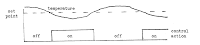
The major disadvantage with this type of control is that the controller

output bears no relationship to the error signal, i.e. the output is

ON/OFF or level 1 or level 2 no matter how high the error. The control

is either non or too much. In addition depending upon the sensitivity

of the system the controller may well cycle at high frequency, e.g. the

boiler being switched ON/OFF very rapidly as the temperature falls

and rises. To prevent this many controllers have ‘backlash’ built in or

have two limits provided. For example a room thermostat may be set

to 700F and due to backlash it will switch on a 680F and off at 720F.

This prevents the boiler being switched ON/OFF very rapidly if the

deviation around the set point was small. In addition theoretical analysis

of such a control system is difficult, i.e. the control action is

discontinuous, and is often treated as two linear problems (i) with the

system ON (ii) with the system OFF.
more

Bang bang control

How much should the software increase or decrease the drive signal?
One option is to just set the drive signal to its minimum value when you
want the plant to decrease its activity and to its maximum value when
you want the plant to increase its activity. This strategy is called on-off
control, and it is how many thermostats work.

On-off control doesn't work well in all systems. If the thermostat waits
until the desired temperature is achieved to turn off the heater,
the temperature may overshoot. See Figure. The same amount of
overshoot and ripple probably isn't acceptable in an elevator.
more

On/off control Index

Control and Automation Home